    Don't know          Legal      No answer Not applicable      Not legal
438 3185 10 3065 2725 Decision Trees and Random Forests
DSC365: Introduction to Data Science
2026-10-27
Announcements
Lab 5 (Linear Models)
- Due Tonight at 11:59 pm in Blueline
Quiz 3: in class on Thursday (October )
- Covers: Prediction/KNN/Tree-Based Methods
- If we don’t get to it in class today, it won’t be on the quiz, but you might need it for the lab.
Tree-based machine learning methods
Tree-Based Methods
- Can be used for both regression and classification
Regression models \(\longrightarrow\) quantitative response variable
Classification models \(\longrightarrow\) categorical response
- These involve stratifying or segmenting the predictor space into a number of simple regions
Example Classification Scenario
Example: Marijuana legalization
The General Social Survey is a wide-ranging survey conducted biannually to measure cultural shifts in American society. We can use the GSS to get an idea of how popular opinion has changed.
Goal: Use Age to predict people’s opinion of marijuana legalization.
Let’s Clean Our Data! Yay!
Data: GSS2016.csv
Data cleaning: decision-trees-random-forests.R
- Let’s only look at one year, say 2016, and remove “Not applicable from our response”
- Want just two groups for responses: Legal and Not legal
- Change variables to proper type
Testing data v. Training data
How many people in the training data set support marijuana legalization?
Decision Trees: Classification
What is a decision tree
Decision trees: A tree-like model of decisions and their possible consequences
- Has flowchart-like structure in which each…
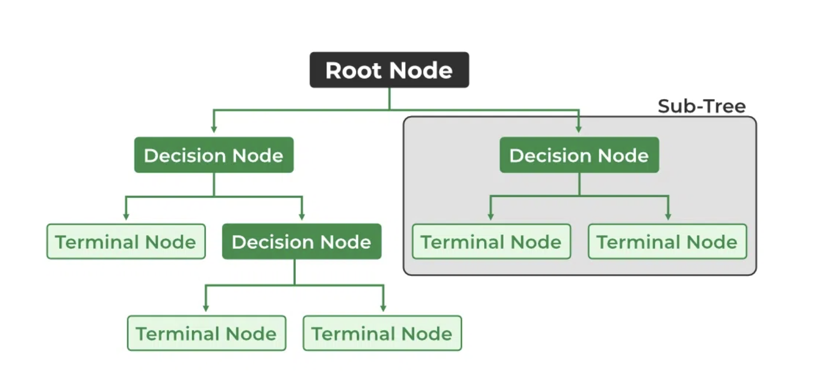
How Decision Trees classify
How to decide to split?
- As the number of predictors increases, so does the number of possible trees.
- Optimal decision trees do not exist (Hyafil & Rivest, 1976)
- So several competing methods for building decision trees
How Decision Trees classify (cont)
Recursive Partitioning: Split infinite # of times until reach stopping criterion.
Split: Gini Index (default): \[G = \sum_{k=1}^{K} \hat{p}_{mk}(1-\hat{p}_{mk})\] where \(\hat{p}_{mk}\) is the proportion of training observations in \(m^{th}\) region from \(k^{th}\) class.
Stop: Complexity parameter
Fitting A Decision Tree (Classification)
n= 1565

node), split, n, loss, yval, (yprob)
      * denotes terminal node

1) root 1565 654 Legal (0.5821086 0.4178914)
  2) AGE< 68.5 1350 521 Legal (0.6140741 0.3859259) *
  3) AGE>=68.5 215  82 Not legal (0.3813953 0.6186047) *
Visualizing a Decision Tree (Classification)
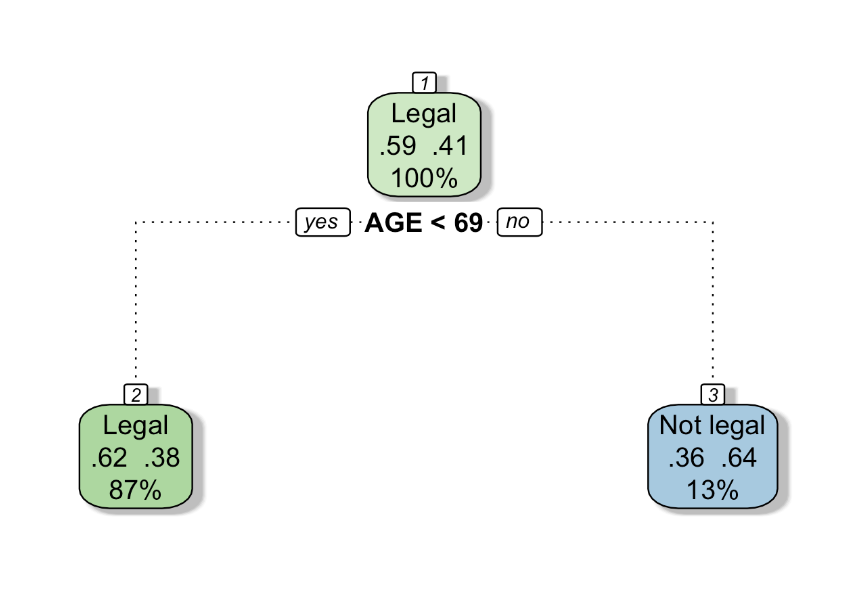
Evaluation
Evaluating a decision tree
- Confusion Matrix
- Classification Accuracy
Evaluating a decision tree: Confusion Matrix
           LEGAL
Legal_Tree  Legal Not legal
  Legal       829       521
Not legal 82 133Evaluating a decision tree: Classification Accuracy
Training Accuracy:
Testing Accuracy:
Tuning Parameter: Complexity parameter
Using recursive partitioning can overfit the training data - Prune Tree
Classification tree:
rpart(formula = LEGAL ~ AGE, data = TRAIN, na.action = na.pass)

Variables actually used in tree construction:
[1] AGE

Root node error: 654/1565 = 0.41789

n= 1565

        CP nsplit rel error  xerror     xstd
1 0.077982      0   1.00000 1.00000 0.029834
2 0.010000 1 0.92202 0.94037 0.029544- Changing complexity parameter:
Decision Trees for Regression
Decision Trees (Regression)
How to decide to split?
- Find regions \((R_j)\) that minimizes the residual sum of squares \[RSS = \sum^{J}_{j=1}\sum_{i \in R_j}(y_i - \hat{y}_{R_j})^2\]
- Stops when you reach some criterion (cp)
Fitting A Decision Tree (Regression)
Let’s suppose we want to use people’s political view (POLVIEWS) and marital status (MARITAL) to estimate people’s age.
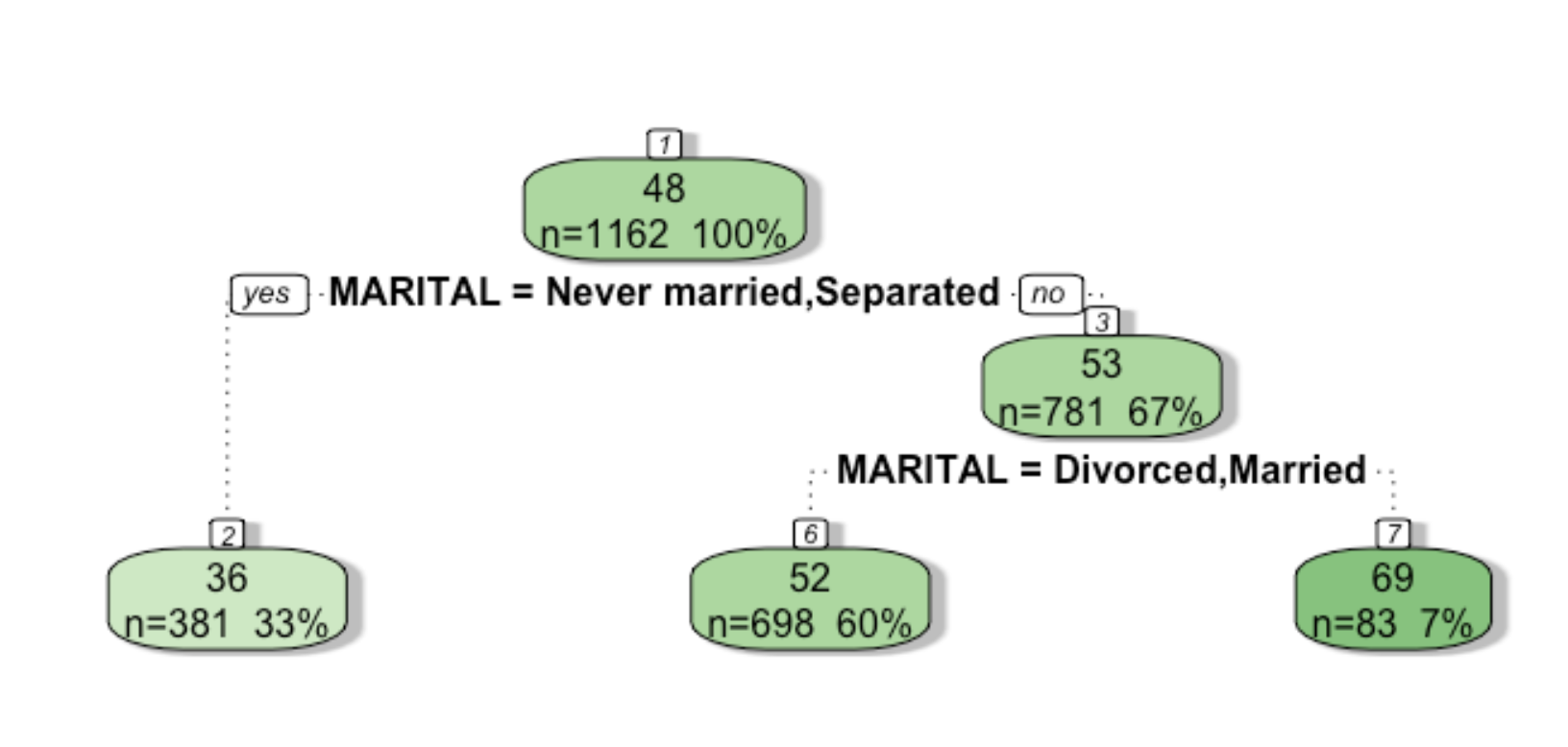
Prediction using Decision Tree
We can still use the predict function to predict our regression decision tree outputs.
       1        2        3        4        5        6
51.93004 51.93004 51.93004 51.93004 35.25934 51.93004
Caution: Can only predict using categorical variables located in the Training Set
Comparison with other methods
Trees Versus Linear Models
- If the relationship between the features and the response is well approximated by a linear model:
- Linear regression
- If instead there is a highly nonlinear and complex relationship between the features and the response as indicated by model:
- Decision trees
Advantages and Disadvantages of Decision Trees
Advantages
Disadvantages
Random Forests
Random Forests
A random forest is collection of decision trees1 that are aggregated by majority rule
When to use random forest:
- large number of variables, no idea which are important
- potential collinearity in predictors
Building a Random Forest
In building a random forest, each time a split in a tree is considered, a random sample of \(m\) predictors is chosen as split candidates from the full set of \(p\) predictors.
- each time a split is considered, a fresh set of \(m\) random predictors are selected
- Only one of the \(m\) variables is selected for the split
- \(m\) is a tuning parameter. Typically use \(m \approx \sqrt{p}\),
Hence, at each split in the tree, the algorithm is not even allowed to consider a majority of the available predictors. Why is this a good thing?
- Roughly speaking, randomness is a method of search: You are searching the space of all possible trees for the “best” or “most explanatory.” So randomly picking variables can help you discover the most important/most explanatory predictors.
Example: Identifying Important Variables
Fit random forest
Goal: Which variables are most important for predicting views on marijuana legalization?
The code below will fit a model to predict LEGAL using all the other variables.
na,action = na.omitignores observations with missing datantree = 201is the number of trees in the forest (odd so there won’t be ties)mtry = 4the number \(m\) of variables to use at each split (note: there’s a total of \(p = 16\) predictors, and \(m = 4 = \sqrt{p} = \sqrt{16}\))
Fit random forest (cont)
Here’s the actual output. Explanation below the output
Call:
 randomForest(formula = as.factor(LEGAL) ~ NEWSFROM + HAPPY +      RELIG + COURTS + ENERGY + EDUC + ENVIR + POLVIEWS + PARTYID +      REGION + INCOME + SEX + DEGREE + AGE + MARITAL + BALLOT,      data = TRAIN, ntree = 201, mtry = 4, na.action = na.omit)
               Type of random forest: classification
                     Number of trees: 201
No. of variables tried at each split: 4

        OOB estimate of  error rate: 33.96%
Confusion matrix:
          Legal Not legal class.error
Legal       704       202   0.2229581
Not legal   325       321   0.5030960
Interpreting the output:
OOB estimate of error rate: 33.96%
For each tree, some of the data is held out (as testing data). This error rate is the average, over those trees, of the test error.
Test predictions
        1         2         3         4         5
Not legal     Legal     Legal     Legal     Legal
Levels: Legal Not legal[1] 0.5717949Classification accuracy above 50% is better than random guessing, but still worse than a decision tree just using AGE
Variable Importance
Since each tree in a random forest uses a different set of variables, we want to keep track of which variables seem to be the most consistently influential.
    rowname MeanDecreaseGini
1       AGE        128.51054
2    REGION         68.41636
3  POLVIEWS         65.99878
4    INCOME         52.25881
5    DEGREE         48.04504
6    COURTS         45.31095
7   MARITAL         44.85723
8     RELIG         44.83231
9   PARTYID         41.61337
10   ENERGY         36.68400
11    HAPPY         35.53879
12    ENVIR         34.43033
13     EDUC         29.67761
14 NEWSFROM         24.74390
15      SEX         22.24408
16   BALLOT         20.41207
Table shows how much the Gini index decreases when a variable is included
From previous slides, we want to minimize Gini index, so the largest decrease corresponds to the most useful variables
Summary
Modeling Data
- Linear model
- The basic model for regression only
- easy interpretation, but strict assumptions
- Use cross-validation (CV) to ensure quality of model
- KNN:
- Can be applied to regression and classification
- fast, no assumptions, can add data anytime.
- large number of variables can lower quality
- use CV to decide \(k\)
- Decision tree:
- Can be applied to regression and classification.
- good data visualization
- high variance
- Random Forest:
- a collection of tree models; can be applied to regression and classification.
- Hard to interpret, but can output variable importance
- Can be useful for variable selection
- outperforms linear model when variables are no linearly independent
Variable Selection
Ultimately, a model is a way to convert input variables into output predictions. Which variables should you use?
Variable Selection is a hard problem
- Variable importance (from a few slides ago) is one way
- the \(R^2\) value from a linear regression is another
A few more methods will come up over the remainder of the semester, but there is no single best way to do it.