k-Nearest Neighbors (KNN)

DSC365: Introduction to Data Science

2026-10-22

Outline

• Classifiers
• \(k\)-Nearest Neighbors
• Examples
• Model Evaluation
• Caveats
• KNN for regression

Announcements

Mini Project 2

• Due Tonight at 11:59 in Blueline

Lab 5 (Linear Models)

• Due next Tuesday (October 27) at 11:59 pm in Blueline

Quiz 3: in class next Thursday, October 29

• Covers: Prediction/KNN/Tree-Based Methods

Source code for today’s slides – don’t forget to comment out the include_graphics lines!

Classifiers

Classification vs. Regression

A model predicts a response variable (\(y\)) from predictor variables (\(x\))

Regression: \(y\) is numeric

Classification: \(y\) is categorical

“Lazy” learning

Lazy learning: no assumptions necessary to classify data

• predicting outcomes without specifying a model

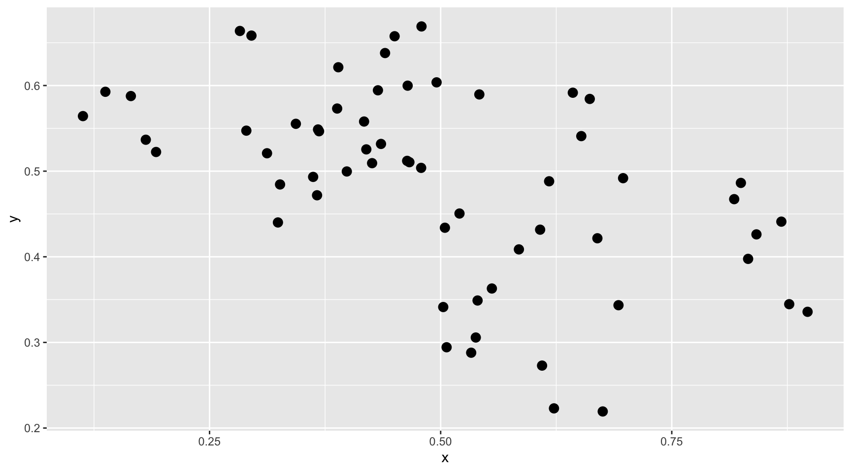
Example: Consider the plot below - describe the relationship between x and y.

“Lazy” learning

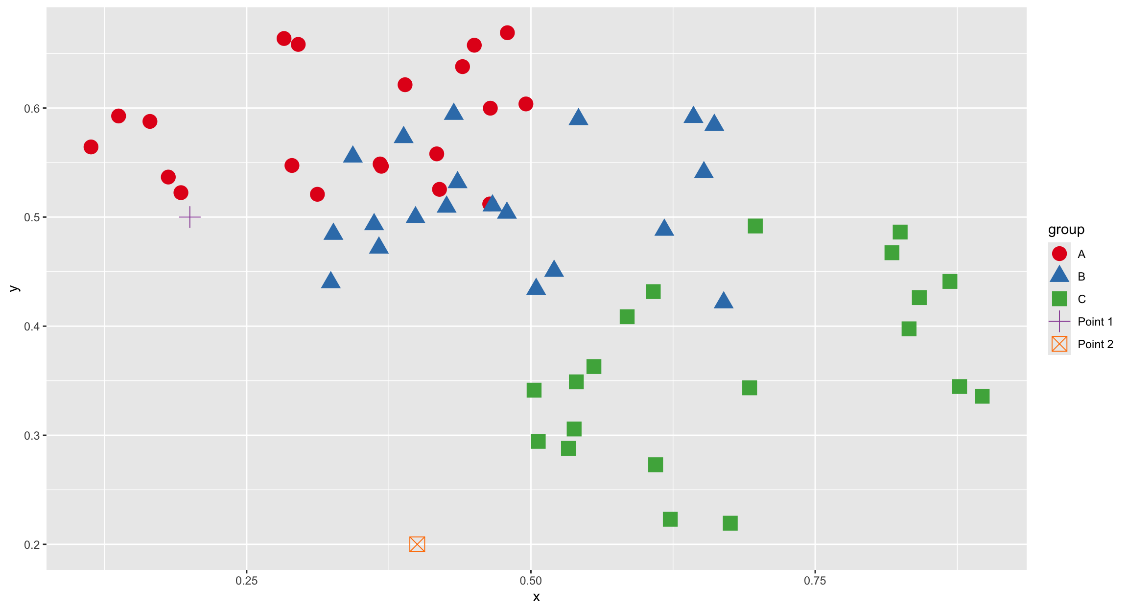
What if the data points belonged to three different groups, like this? How should a new data point, \((0.2, 0.5)\) be classified? What about \((0.4, 0.2)\)?

\(k\)-Nearest Neighbors

Bayes Classifier

A good classifier minimizes Testing Error (fraction of mis-classified observations)

• Bayes Classifier produce the lowest possible test error rate (proof)

Bayes Classifier assigns each observation to is most likely class using:

\[P(Y = j|X = x_0)\]

Problems:

• We don’t know the conditional probability distribution, so we have to estimate it

• (also, even if we did know the distribution, it could lead to overfitting)

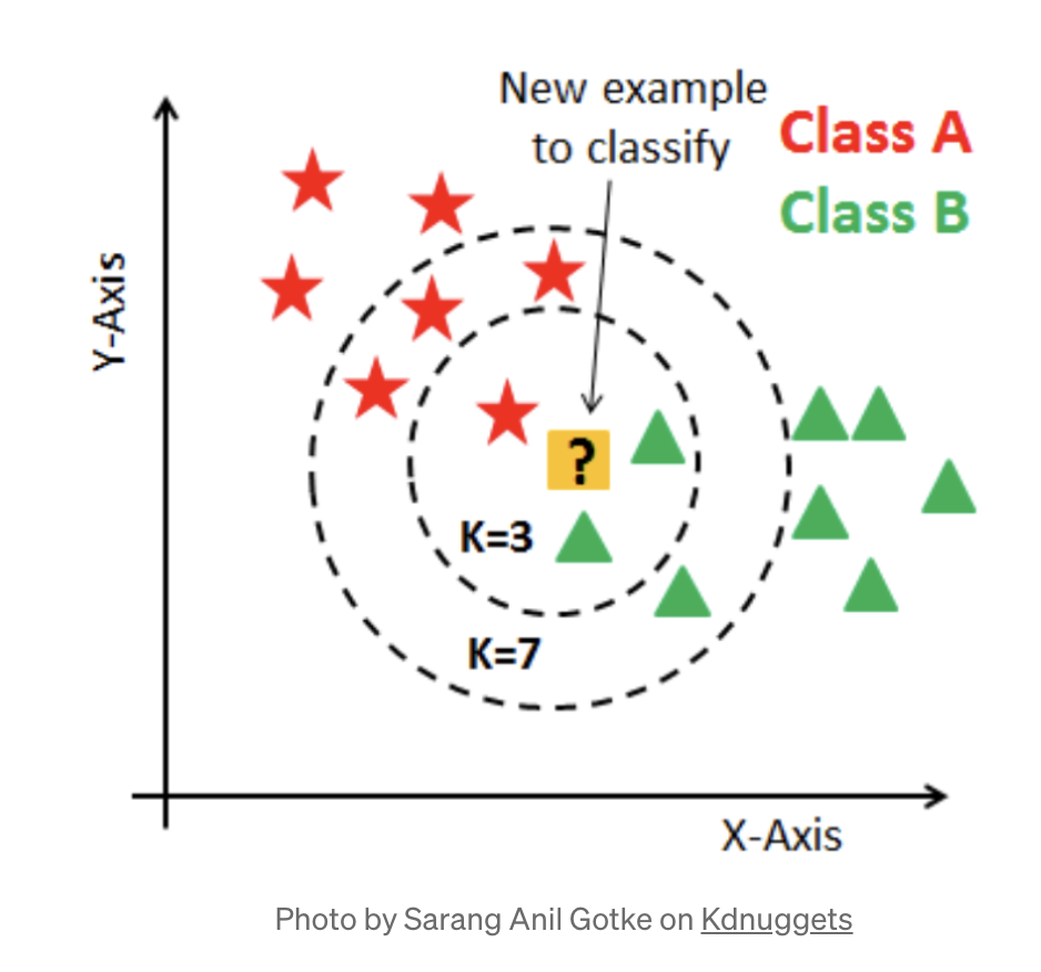
\(k\)-nearest neighbor (KNN) classifier:

A non-parametric supervised learning method that estimates the conditional probability.

Output: group membership of new point

• if k = 3 -> A, if k = 7 -> B. Sensitive to \(k\)!

• membership is most common among the closest \(k\) training points

• Theoretically, if we choose \(k\) well, it becomes close to a Bayes classifier.

KNN classification algorithm

Input/set up: Training data is labeled

Algorithm: Given a new data point, these steps output its membership:

1. Choose a value for \(k\) (see note¹)

2. find the \(k\) nearest neighbors to that point (from the training data)

3. From among those \(k\), count the # in each category

4. Assign new point based on plurality vote (i.e. the highest number)

1. \(k\) is a tuning parameter or hyperparameter: It is a choice we make, rather than an inferred property of the population

knn() function

Example: Let’s classify our new points

library(class)

\(k=2\)?

knnMod1 = knn(train=data[,1:2], 
          test = new.pts[,1:2], 
          cl = data$group, 
          k = 2, prob = TRUE)
knnMod1

[1] A C
attr(,"prob")
[1] 1 1
Levels: A B C

\(k=10\)?

knnMod2 = knn(train =data[,1:2], 
          test = new.pts[,1:2], 
          cl = data$group, 
          k = 10, prob = TRUE)
knnMod2

[1] A C
attr(,"prob")
[1] 0.7 0.8
Levels: A B C

Advantages and Disadvantages of KNN

Advantages:

1. It’s easy! (especially in R!)
2. You don’t have to check any assumptions about the data

Disdvantages:

1. Hard to decide \(k\) (typically, you’ll need to try several different values)
2. Need \(n\) (number of observations) to be large relative to \(p\) (number of predictors)
3. The geometry of the data affects the quality of fit (i.e. if the data is clustered, KNN does better)
4. Because it uses distance, it only works with numeric predictors (unless we encode qualitative variables as dummy variables like in Linear Regression, which comes with its own geometry issues)

Choice of \(k\)

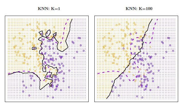
(in this example), \(k = 1\) leads to low bias (the boundary is close to the dashed purple line, which is the true boundary between classes), but high variance. On the other hand, \(k = 100\) leads to high bias (the boundary is far from the true boundary), but lower variance.

Examples

Example: Credit Utilization

Predict which utilization quantile a new customer falls into based on their application data (credit rating and age).

Name	Age	Credit Rating
Lacey	33	750
Zach	47	400
Ashlee	21	250

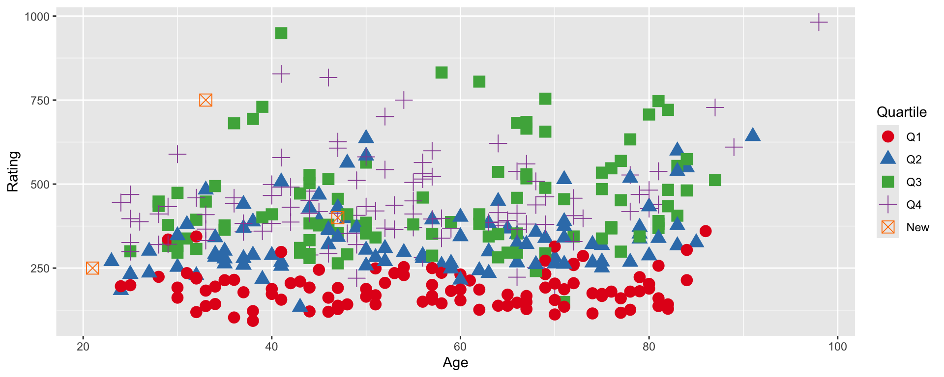
Example: Credit Utilization

\(k=20\)?

knn20 = knn(train = old[,1:2],
            test = apps[,1:2],
            cl = old[,3], 
            k = 20, prob = TRUE)
knn20

[1] Q3 Q4 Q2
attr(,"prob")
[1] 0.65 0.40 0.65
Levels: Q1 Q2 Q3 Q4

\(k=100\)?

knn100 = knn(train = old[,1:2],
            test = apps[,1:2],
            cl = old[,3], 
            k = 100, prob= TRUE)
knn100

[1] Q4 Q4 Q2
attr(,"prob")
[1] 0.44 0.46 0.45
Levels: Q1 Q2 Q3 Q4

Model Evaluation

Example: Credit utilization

Is KNN an effective predictor of quartile using an applicant’s age, credit rating, income, number of existing credit cards, and education level?

Example: Credit utilization (cont)

Randomly selected 100 observations for testing, assigned the other 300 to training set.

set.seed(365)
test_ID = sample(1:nrow(Credit), size = 100)
TEST = Credit[test_ID,]
TRAIN = Credit[-test_ID, ]

#only select variables we want
knn_train = TRAIN %>% dplyr::select(Age, Rating, Income, 
                                    Cards, Education)
knn_test = TEST %>% dplyr::select(Age, Rating, Income, 
                                  Cards, Education) 

knn50 = knn(train = knn_train, 
            test = knn_test,
            cl = TRAIN$Quartile, 
            k = 50, prob = TRUE)
knn50

  [1] Q4 Q1 Q4 Q1 Q4 Q3 Q4 Q4 Q1 Q4 Q2 Q2 Q4 Q4 Q3 Q1 Q1 Q3 Q4 Q1 Q4 Q2 Q3 Q2 Q2
 [26] Q4 Q3 Q4 Q4 Q2 Q2 Q2 Q3 Q2 Q1 Q4 Q4 Q3 Q3 Q2 Q1 Q2 Q3 Q4 Q1 Q4 Q3 Q2 Q4 Q4
 [51] Q4 Q2 Q4 Q1 Q4 Q1 Q1 Q2 Q1 Q1 Q1 Q4 Q1 Q4 Q4 Q1 Q4 Q4 Q4 Q4 Q2 Q1 Q4 Q2 Q3
 [76] Q2 Q2 Q1 Q1 Q4 Q2 Q4 Q2 Q3 Q2 Q4 Q1 Q4 Q4 Q2 Q4 Q4 Q4 Q4 Q2 Q2 Q4 Q2 Q1 Q2
attr(,"prob")
  [1] 0.66 0.86 0.54 0.96 0.50 0.40 0.36 0.52 0.96 0.66 0.54 0.56 0.54 0.42 0.38
 [16] 0.96 0.92 0.42 0.46 0.98 0.44 0.52 0.40 0.54 0.60 0.46 0.46 0.42 0.62 0.52
 [31] 0.52 0.56 0.40 0.54 0.58 0.46 0.52 0.38 0.46 0.52 0.96 0.44 0.44 0.42 0.98
 [46] 0.50 0.44 0.48 0.54 0.46 0.50 0.58 0.46 0.90 0.50 0.94 0.96 0.42 0.96 0.82
 [61] 0.54 0.48 0.54 0.58 0.44 0.96 0.44 0.46 0.58 0.54 0.34 0.96 0.44 0.58 0.42
 [76] 0.34 0.54 0.96 0.96 0.42 0.60 0.52 0.56 0.40 0.48 0.54 0.64 0.34 0.60 0.56
 [91] 0.44 0.50 0.48 0.50 0.46 0.52 0.44 0.58 0.78 0.58
Levels: Q1 Q2 Q3 Q4

Evaluation: Classification Accuracy

Now, we’ll set the testing data as “new data”, and make predictions using the k-nearest neighbors from the training data.

#Create Confusion Matrix - Base R
t = table(knn50, TEST$Quartile)
t

     
knn50 Q1 Q2 Q3 Q4
   Q1 18  2  1  1
   Q2  4 16  5  1
   Q3  0  3  7  2
   Q4  0  8 16 16

sum(diag(t))/nrow(TEST) #Classification Accuracy

[1] 0.57

Try it yourself!

set.seed(365)
test_ID = sample(1:nrow(Credit), size = 100)
TEST = Credit[test_ID,]
TRAIN = Credit[-test_ID, ]

#only select variables we want
knn_train = TRAIN %>% dplyr::select(Age, Rating, Income, 
                                    Cards, Education)
knn_test = TEST %>% dplyr::select(Age, Rating, Income, 
                                  Cards, Education) 

our_choice_of_k = 17

knnk = knn(train = knn_train, 
            test = knn_test,
            cl = TRAIN$Quartile, 
            k = our_choice_of_k, prob = TRUE)

t = table(knnk, TEST$Quartile)
sum(diag(t))/nrow(TEST)

[1] 0.61

Caveats

Scaling Data

knn_train_scale <- knn_train %>% scale()
knn_test_scale <- knn_test %>% scale()

knn50_scale = knn(train = knn_train_scale, 
            test = knn_test_scale,
            cl = TRAIN$Quartile, 
            k = 50, prob = TRUE)


t_scale = table(knn50_scale, TEST$Quartile)

sum(diag(t_scale))/nrow(TEST) #Classification Accuracy

[1] 0.43

1. Draw a circle with radius 1 centered at the point \((1,1)\) in the \(x\)-\(y\) plane. Do the same for the points \((1,-1)\), \((-1,-1)\), and \((-1,1)\).
2. Draw a circle, centered at the origin, that is lies between all four circles, and and is tangent to them. What is its radius?
3. It’ll be tricky, but try to imagine this same process with spheres in 3D space – now with 8 of them, one at each corner of a cube. What is the radius of the sphere that lies nestled in the middle?
4. What if you do this in 4 dimensions? 5? 6? What strange thing happens in 10 dimensions?

KNN for regression

KNN Regression algorithm

KNN can also predict quantitative responses - alternative to Linear Regression¹

1. Choose a value for \(k\) (same as last time)

2. find \(k\) nearest neighbors (same as last time)

3. Response value for new point is average of the response values for the \(k\) nearest points (that is, \(f(x_0) = \frac1k \sum_{j=1}^k f(q_j))\), where the \(q_1,q_2,\dots,q_k\) are the \(k\) nearest training points)

Notes: Small \(k\) will perfectly interpolate the data, while large \(k\) will smooth the data

1. Worried your data doesn’t satisfy the LINE assumptions? This may be a good option for mini project 3!

Example: Credit Utilization

knn_train = TRAIN %>% dplyr::select(Age, Rating, Income, Cards, 
                                    Education)
knn_test = TEST %>% dplyr::select(Age, Rating, Income, Cards, 
                                  Education) 

knn50 = FNN::knn.reg(train = knn_train, 
            test = knn_test,
            y = TRAIN$Utilization, 
            k = 50)

head(knn50$pred, n = 5)

[1] 0.157343839 0.011478125 0.144051032 0.005360386 0.142495141

Metrics::rmse(TEST$Utilization, knn50$pred)

[1] 0.0386645

Is this good? Compare with (1) spread of response variable itself, (2) RMSE from other methods (e.g. linear regression)

Linear Regression vs KNN Regression

Parametric vs. nonparametric methods:
- If your model is correct (e.g. you are using linear regression to model a relationship that truly is linear), parameteric methods will outperform nonparametric every time.

Linearity:
- Many relationships in data are actually nonlinear, so KNN regression may outperform Linear Regression (e.g. the RMSE from KNN might be lower than from LR)

Curse of Dimensionality:
- Each observation is represented as a point in \(p\)-dimensional space (where \(p\) is the number of predictors). High-dimensional geometry is weird¹, and in particular, when \(p\) is large, individual points will tend to be farther apart. As such, even if your data is nonlinear, Linear Regression may do better than KNN when \(p\) is large.

In situations where the relationship is nonlinear, KNN regression may perform better than Linear Regression

1. see the speaker notes on the Scaling Data slide