Cross Validation
2026-10-20
Announcements
Mini Project 2
- Due this Thursday, October 22, 11:59pm in Blueline
Lab 5 (Linear Models)
- Due next Tuesday October 27 at 11:59 pm in Blueline
Quiz 3: in class next Thursday October 29
- Covers: Prediction/KNN/Tree-Based Methods
Branches of Machine Learning
Machine Learning: a broad term, coined in the 1950s, describing a set of inter-related techniques for extracting info from data
Supervised Learning: Modeling a specific response from “labeled” data. That is, we have a set of input-output pairs.
Unsupervised Learning: Approach to finding patterns where there is no clear response variable.
Models
Prediction
There are two things we can do with fitting a model:
- Interpretation
- Prediction
Calculating a prediction is easy: Plug in your predictor variables into the formula defining the model to get the predicted response \(\hat{y}\)
Getting a good prediction is hard:
No one model is “best”
“All models are wrong, but some are useful”
- Prediction Accuracy and Model Interpretability Trade-Off
- simple models are easy to interpret (e.g. coefficients of a linear regression), but might not be accurate for more complex data.
- complicated models can be more accurate, but no one knows what any particular parameter does.
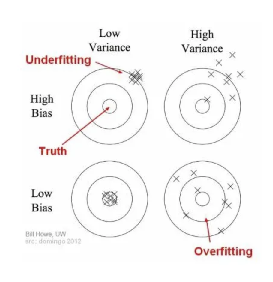
- Bias vs Variance Trade-Off
- we generally want low bias, low variance.
- But mathematically, these are often mutually incompatible goals.
Bias vs Variance
Over vs Under Fitting
Splitting Data
Test vs. Train
Several steps to create a useful statistical model: parameter estimation, model selection, performance assessment, etc.
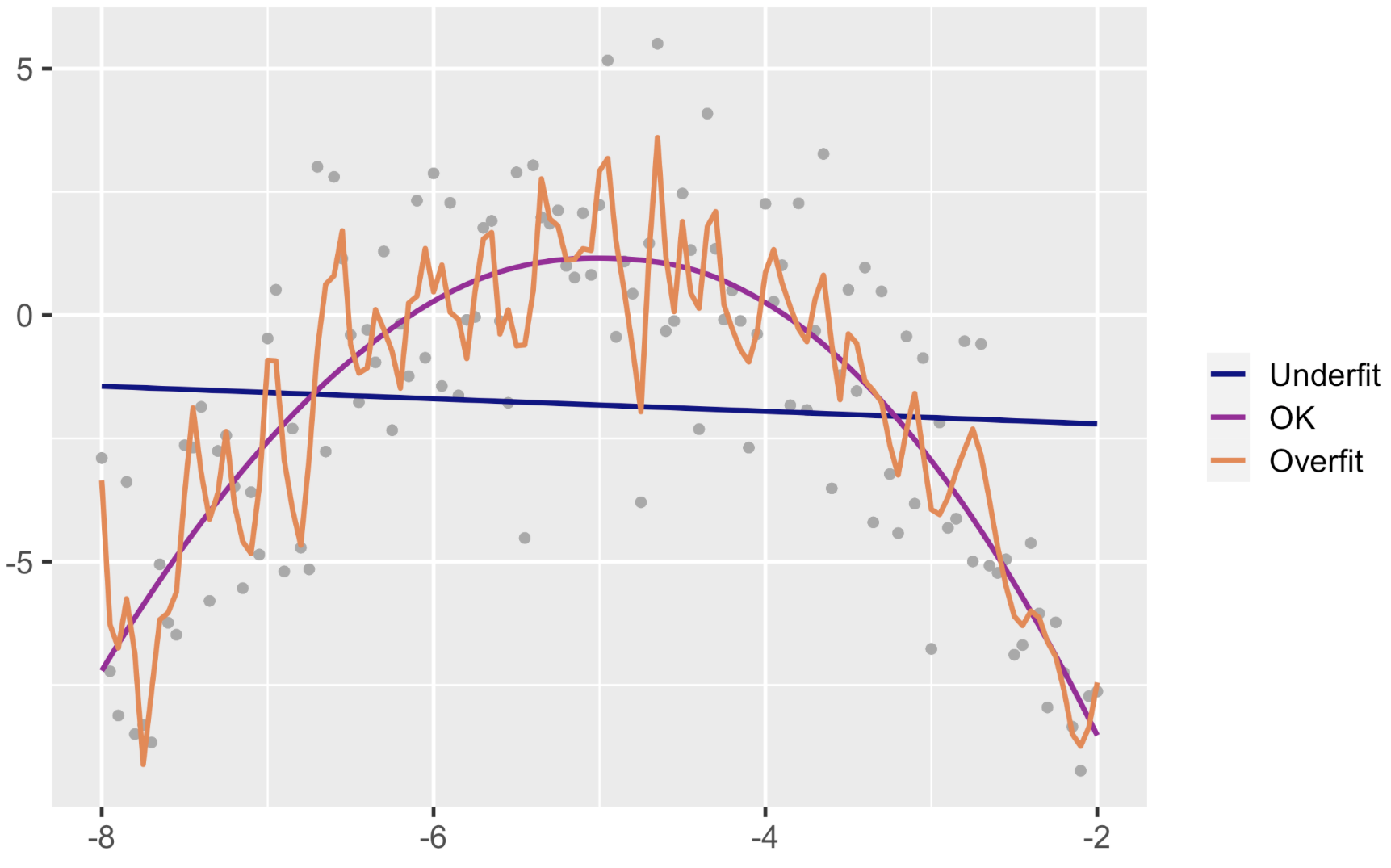
Doing all of this on the entire data we have available can lead to overfitting
To avoid overfitting, we split the data.
- split the data into TEST and TRAIN
- That is, we fit the model to the training data (TRAIN) and then measure the “quality” of the model on the testing data (TEST)
Example: Flight Data
Consider a random sample of 1000 flights from NYC to Chicago in 2013. We want to create a model to predict arrival delay.
- Split it into a training and a testing set.
Example: Flight Data
- Fit model to Training set:
This finds the coefficients in the model \(y = \beta_0 + \beta_{hour} X_{hour} + \beta_{dep delay} X_{dep delay}\)
- Predict outcome on the Testing Set:
         1          2          3          4          5          6
 -9.759234 -13.193375 -15.259597 -14.309398 -20.313551  -6.659900
Plugs all of the TEST values of hour and dep_delay into the model above
Model evaluation
Is that right?
We can compare the predicted values to the actual values:
Evaluate Performance: RMSE
Root Mean Square Error (RMSE) - for numerical response
\[ \text{RMSE} = \sqrt{\frac{\sum^{n}_{i=1}(y_i - \hat{y}_i)^2}{n}} \]
RMSE for Test Set:
Penalizes large errors more heavily (because error is squared), so it’s sensitive to outliers.
To give the number meaning, compare it to, say, the standard deviation in the arrival delays
The RMSE (15.8) is smaller than the standard deviation of the response variable (47.1), which is a good sign
Evaluate Performance: MAE
Mean Absolute Error (MAE) - for numerical response
\[\text{MAE} = \frac{1}{n} \sum^{n}_{i=1}|y_i - \hat{y}_i|\]
MAE for Test Set:
Model Comparison
# A tibble: 1 × 2
    MSE1   MSE2
   <dbl>  <dbl>
1 15.854 15.844# A tibble: 1 × 2
MAE1 MAE2
<dbl> <dbl>
1 12.031 12.046Cross Validation
Problems with single splits
Potential Problem with a single split into training/testing: you evaluated the model only once and you are not sure your good result is by luck or not
- when the data set is small, the chances we were lucky is higher (i.e. for very large data sets, there’s usually less of a need for extensive cross-validation)
- Basically, we want to evaluate the model multiple times to be confident in the fit.
We can easily do this using cross validation
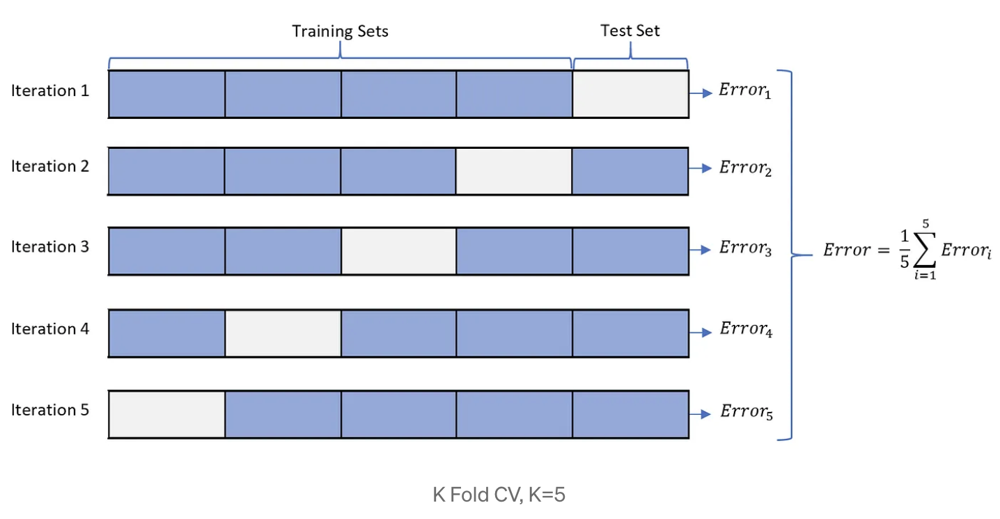
- A resampling method that uses different portions of the data to test and train a model on different iterations
\(k\)-fold Cross Validation
- Split the dataset into \(k\) subsets randomly
- Generally choose \(k = 5\) or \(k = 10\).
- Use k-1 subsets for training the model
- Test the model against that one subset that was left in the previous step
\(k\)-fold Cross Validation in R
Linear Regression

1000 samples
   2 predictor

No pre-processing
Resampling: Cross-Validated (5 fold)
Summary of sample sizes: 800, 800, 800, 800, 800
Resampling results:

  RMSE     Rsquared   MAE
  19.0237  0.8312302  13.36263

Tuning parameter 'intercept' was held constant at a value of TRUE
Dealing with Hyperparameters
If your model has hyperparameters, best to do it this way:
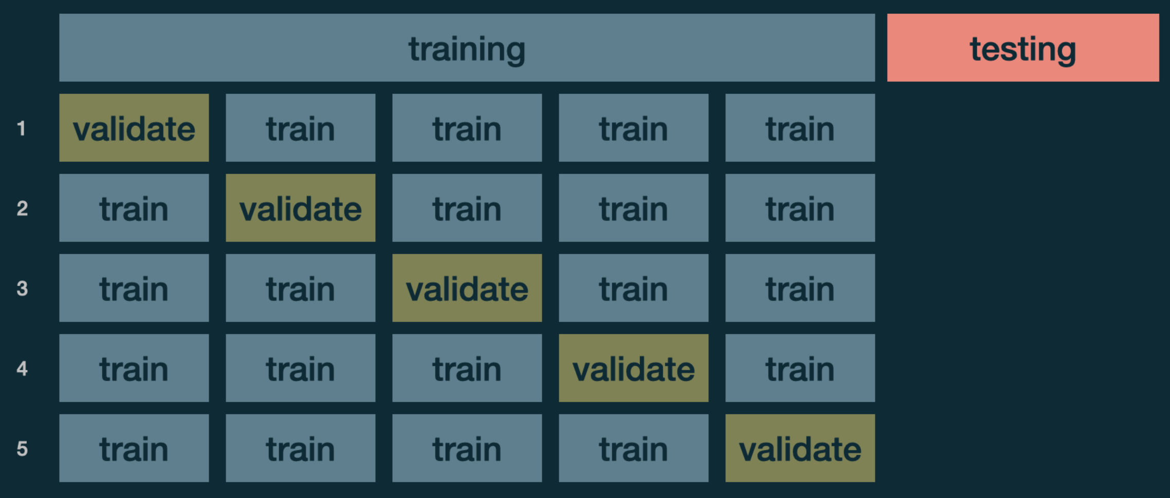
Withhold a portion of the data for testing, and then do cross-validation within the testing set
Note: Linear regression does not have hyperparameters, but we will discuss methods that do later in the course.
Caveats
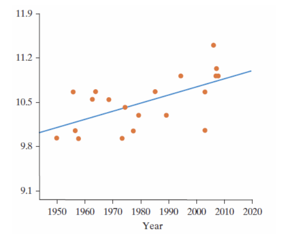
Caution with Linear Models: Extrapolation
We extrapolate when we use the regression equation to produce a response value from an x-value that is outside the range of the observed x-values
Example: Relationship between year and diameter of a dinner plate.