Principal Component Analysis (PCA)

DSC365: Introduction to Data Science

2026-11-05

Announcements

Lab 6

  • Due Tuesday November 10 at 11:59 pm in Blueline

Mini Project 3

  • Instructions posted here
  • Due Thursday November 12 Tuesday, November 17 by 2:00pm in Blueline (peer review during class)

DSC 465: Machine Learning will not be offered in the 2027-2028 school year. It will be offered in Spring 2027 (next semester) and the next time will be Fall 2028

Upcoming Talk about Sports Analytics next Friday at 7pm in Hixson-Lied G04. See flyer on Blueline for more details.

Modern Data Science with R, Chapter 12

Interactive Walk Through

What is Principal Component Analysis?

These slides: (qmd) (pdf) (data - happyplanet2016.xlsx)

Principal Component Analysis (PCA)

PCA on one foot

Project onto the directions of greatest variance

Principal Component Analysis (PCA): Why?

Sometimes a data set has a lot of variables.

  • Some of these variables carry lots of information.
  • Others carry little to no information.

PCA can help reduce the dimensionality of data by summarizing most of the variation into fewer dimensions, called components.

Principal Component Analysis (PCA): What?

PCA:

Don’t Panic But It’s Time For Linear Algebra

Outlining the idea

  • Our data has \(p\) features, \(X_1,\dots,X_p\)
  • A linear combination of features is a new variable \(Z = \phi_1X_1 + \phi_2X_2 + \cdots + \phi_pX_p\) (each \(\phi_j\) is just a number)
  • Notice that \(Z\) is a new numerical variable, so we can compute its variance. Different choice of \(\phi_j\)s will give different variance
  • Key idea: we can find \(\phi_j\)s (under some constraints) to maximize variance of \(Z\)
    • that is the first principal component

Picture Time!

PCA: How?

1).


2).

PCA: How? (2/3)

  1. Find Principal Components. Features are \(X_1, \dots X_p\).
  • First Principal Component: \(Z_1 = \phi_{11}X_1 + \phi_{21}X_2 + \cdots + \phi_{p1}X_p\)
    • Choose \(\phi_{j1}\)s to maximize variance of \(Z_1\)
    • Normalized: \(\sum^p_{j=1} \phi^2_{j1} = 1\)
    • optimization problem: \(\text{maximize}_{\phi_{11}, \dots \phi_{p1}}(\frac{1}{n}\sum^{n}_{i=1}(\sum^{p}_{j=1}\phi_{j1}x_{ij})^2)\)
    • the \(\phi_{jk}\)s are called loadings
  • Second Principal Component: maximal variance out of all linear combinations that are uncorrelated (that is, orthogonal) with \(Z_1\)

  • \(k\)th principal component maximizes variance while orthogonal to first \(k-1\) components.

PCA: How? (3/3)

4). Select the number of components that capture most of the variation

Example

Example: Data

The Happy Planet Index is a measure of a country’s ecological and societal “well-being”.

library(readxl)
happyplanet2016 <- read_excel("happyplanet2016.xlsx")
glimpse(happyplanet2016)
1
See announcements slide for data
Rows: 140
Columns: 11
$ Country                 <chr> "Costa Rica", "Mexico", "Colombia", "Vanuatu",…
$ Region                  <chr> "Americas", "Americas", "Americas", "Asia Paci…
$ Life_Expectancy         <dbl> 79.076, 76.411, 73.673, 71.341, 75.477, 77.215…
$ Well_Being              <dbl> 7.30, 7.30, 6.40, 6.47, 5.50, 6.90, 5.40, 4.70…
$ Happy_Life_Years        <dbl> 48.17479, 44.26208, 35.07089, 34.89575, 32.770…
$ Environmental_Footprint <dbl> 2.840000, 2.890000, 1.870000, 1.862620, 1.6500…
$ Inequality              <dbl> 0.14556769, 0.18769899, 0.23504395, 0.22333185…
$ HappyPlanetIndex        <dbl> 44.71407, 40.69729, 40.69501, 40.57010, 40.307…
$ GDP_PC                  <dbl> 9733.3969, 9703.3710, 7885.0613, 3158.4210, 17…
$ Population              <dbl> 4654148, 122070963, 46881018, 247498, 88809200…
$ GINIindex               <dbl> 48.61, 48.07, 53.54, NA, 38.70, 51.90, NA, NA,…
Can we distill this down to a few important variables or ideas?

Example: Fitting PCA

The Happy Planet Index is calculated using a weighted average of these variables. It wouldn’t make sense to try to find linear combinations with a variable that’s already a linear combination, so we remove it.

How are the other variables related?

happyplanet2 <- na.omit(happyplanet2016[,-8])

#scale and find covariance matrix as part of function
happy_pca <- prcomp(x=happyplanet2[,3:10],
                    center=TRUE, scale=TRUE)

summary(happy_pca) #proportion of variance explained
1
Drop column 8, as well as na values
2
Shift the data so it’s mean 0 and then standardize
Importance of components:
                          PC1    PC2     PC3     PC4     PC5     PC6     PC7
Standard deviation     2.2065 1.1417 0.82049 0.76101 0.56043 0.45619 0.21980
Proportion of Variance 0.6086 0.1629 0.08415 0.07239 0.03926 0.02601 0.00604
Cumulative Proportion  0.6086 0.7715 0.85566 0.92805 0.96731 0.99332 0.99936
                           PC8
Standard deviation     0.07136
Proportion of Variance 0.00064
Cumulative Proportion  1.00000

Fitting PCA: Loadings

happy_pca$rotation #loadings
                                PC1         PC2          PC3         PC4
Life_Expectancy         -0.39386299 -0.10210804 -0.005109106 -0.46521889
Well_Being              -0.38084138 -0.32767032 -0.236721404 -0.06883676
Happy_Life_Years        -0.43456875 -0.17515821 -0.093807637 -0.14622457
Environmental_Footprint -0.35028972  0.15469868 -0.069976648  0.68939169
Inequality               0.42016186 -0.02650942 -0.265323358  0.24342252
GDP_PC                  -0.39270248  0.03324252 -0.206237022  0.38291281
Population               0.04745023 -0.72676475  0.613698554  0.27584809
GINIindex                0.23510880 -0.54552656 -0.663840464  0.01488121
                                PC5         PC6         PC7         PC8
Life_Expectancy          0.47756080  0.31566633  0.52567156  0.11811449
Well_Being              -0.48587423 -0.41963145  0.16977285  0.49581180
Happy_Life_Years        -0.22281747 -0.12290385 -0.02778462 -0.82750416
Environmental_Footprint  0.45029109 -0.36263209  0.19392271 -0.03657425
Inequality              -0.29036909  0.15160670  0.73955922 -0.19713856
GDP_PC                  -0.24970437  0.73603463 -0.19285020  0.11930350
Population               0.02363929  0.11234909  0.05877270 -0.01442327
GINIindex                0.36908932  0.01740502 -0.26244106 -0.02852801

Fitting PCA: Number of Components

How many components should we choose?

#install.packages("factoextra")
library(factoextra)
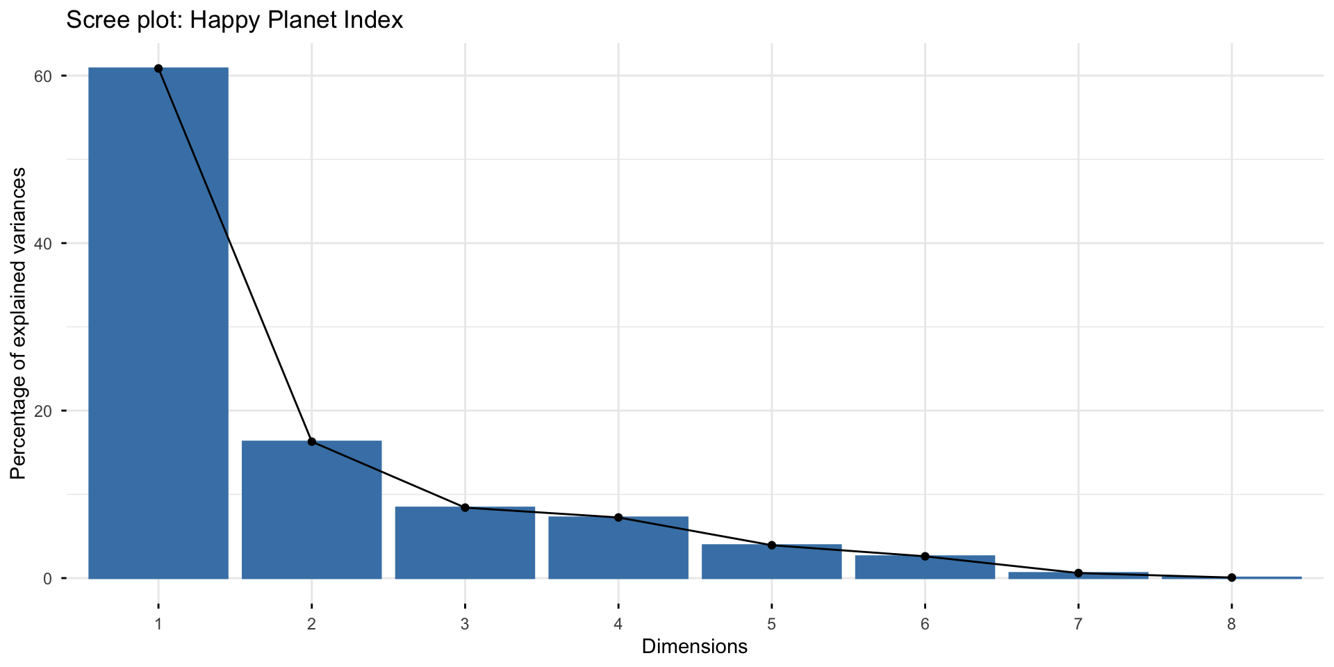
fviz_eig(happy_pca, main = "Scree plot: Happy Planet Index")
Scree plot for the principal components of the Happy Planet Data. The first PC explain roughly 60 percent of the variation, with the second PC around 17 percent. At this point the elbow flattens, so only need the first two PCs

Visualizing

Biplot

A biplot shows the relationships between the components by projecting to plane spanned by two principal components (by default, first two)

  • Perpendicular vectors:

  • Two variables in the same direction:

  • Two variables in the opposite direction:

Biplot (2/2)

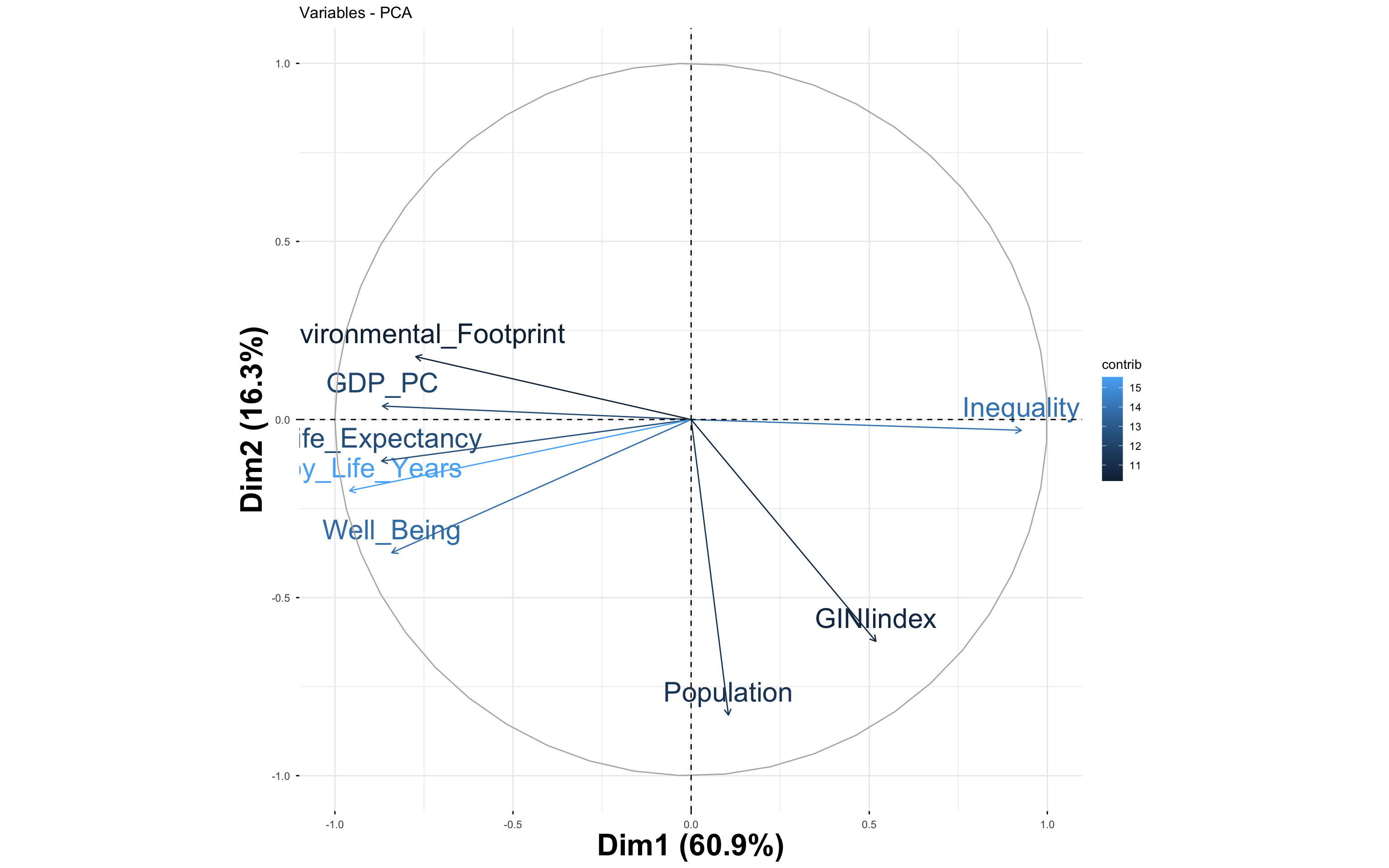
fviz_pca_var(happy_pca, col.var = "contrib")
Biplot of the first two PCs for the Happy Planet Data

ggbiplot

Package available on GitHub – see installation instructions on last slide.

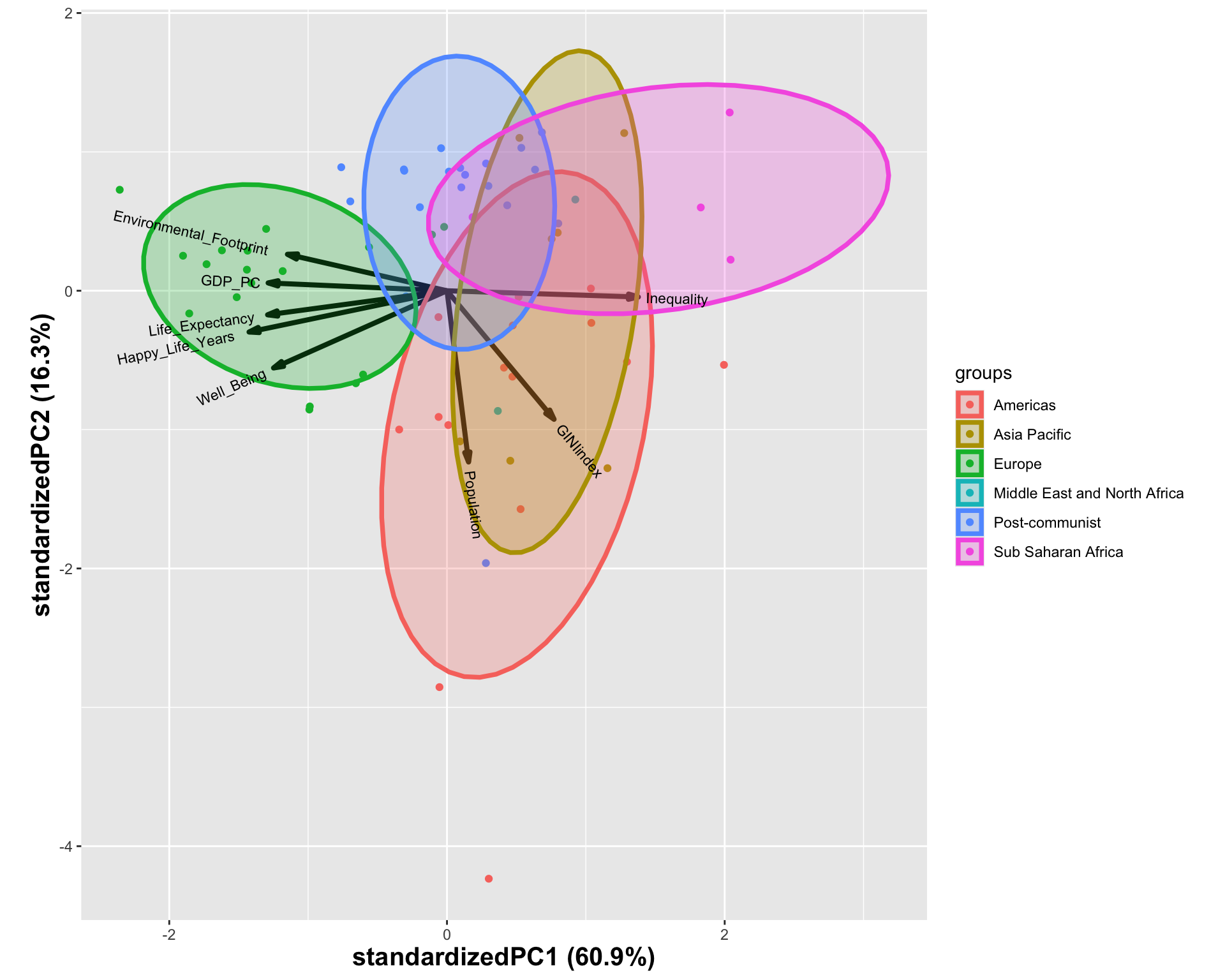
ggbiplot(happy_pca, groups=happyplanet2$Region, ellipse=TRUE)
1
Jump to the last slide for installation instructions for the ggbiplot package.
Biplot of the first two PCs for the Happy Planet Data. Now additionally the observations are on the plot given their relation to PC1 and PC2. The points are then colored by Regions to see if regions are related to how observations hang on the first two PCs

ggbiplot (2/2)

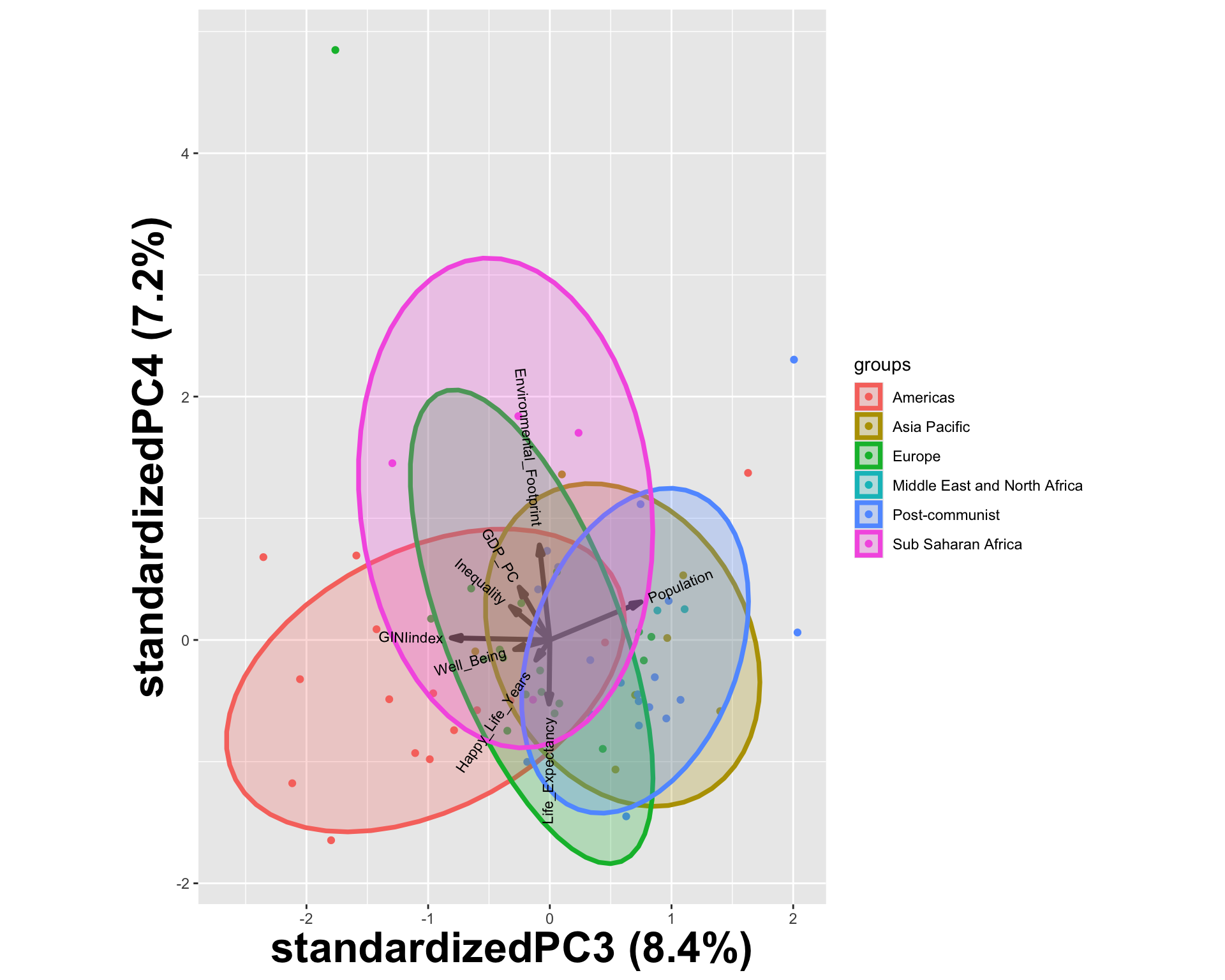
Can also visualize other PCs besides the first two.

ggbiplot(happy_pca, groups=happyplanet2$Region, ellipse=TRUE, 
         choices=c(3,4))
Biplot of the third and fourth PCs for the Happy Planet Data. Now additionally the observations are on the plot given their relation to PC3 and PC4. The points are then colored by Regions to see if regions are related to how observations hang on the first two PCs

Summary

Advantages:


Disadvantages:


Try It Yourself

Try the PCA with the gapminder data. Use all four variables (infant_mortality, life_expectancy, fertility and popualtion) try to make a data visualization to show the relations between the variables.

Danger Zone

Warning

Only do this if you trust the github repo. Doing this with random packages you find online is generally a bad idea.

If a package you might want to use is on GitHub and you know the user’s Git repository: install the package using the install_github function in the devtools library.

library(devtools)
install_github("vqv/ggbiplot")
library(ggbiplot)