Cluster Analysis

DSC365: Introduction to Data Science

2026-11-03

IT IS ELECTION DAY. VOTE.

Announcements

Lab 6

  • Due Tuesday November 10 at 11:59 pm in Blueline

Mini Project 3

  • Due Thursday November 12 by 2:00pm in Blueline (peer review during class)

Suggested reading: Modern Data Science with R, Chapter 12

Link to slide .qmd source
Link to slide pdf

Unsupervised Learning Methods

Supervised vs. unsupervised

Supervised learning has labeled training data

Unsupervised learning

Clustering vs. Principal Components

1). Today: Clustering


2). Thursday: Principal Components

Cluster Analysis

Running example: gapminder

Goal:

Data: Focus on year 2015

library(dslabs)
gapminder_2015 <- gapminder %>%
  filter(year == 2015)
glimpse(gapminder_2015)
Rows: 185
Columns: 9
$ country          <fct> "Albania", "Algeria", "Angola", "Antigua and Barbuda"…
$ year             <int> 2015, 2015, 2015, 2015, 2015, 2015, 2015, 2015, 2015,…
$ infant_mortality <dbl> 12.5, 21.9, 96.0, 5.8, 11.1, 12.6, NA, 3.0, 2.9, 27.9…
$ life_expectancy  <dbl> 78.00, 76.40, 59.60, 76.40, 76.50, 74.70, 75.72, 82.3…
$ fertility        <dbl> 1.78, 2.71, 5.65, 2.06, 2.15, 1.41, 1.66, 1.88, 1.50,…
$ population       <dbl> 2896679, 39666519, 25021974, 91818, 43416755, 3017712…
$ gdp              <dbl> NA, NA, NA, NA, NA, NA, NA, NA, NA, NA, NA, NA, NA, N…
$ continent        <fct> Europe, Africa, Africa, Americas, Americas, Asia, Ame…
$ region           <fct> Southern Europe, Northern Africa, Middle Africa, Cari…

Clustering Techniques

Hierarchical vs. Non-hierarchical

1). Hierarchical Clustering:

  • Example Method:

2). Non-Hierarchical Clustering:

  • Example Method:

\(K\)-Means Clustering

Hierarchical Method: \(K\)-Means Clustering

Overview: partitions the data into a pre-specified number, \(K\), of non-overlapping clusters

Properties:

\(K\)-Means Clustering: Algorithm

Idea: Good clustering means within cluster variation is as small as possible

\[\text{minimize} \left(\sum^K_{j=1}W(C_j)\right)\]

  • \(C_1,\dots, C_K\):

  • \(W(C_j)\):

\(K\)-Means Clustering: Algorithm (2/4)

Problem: very difficult minimization problem as almost \(K^n\) ways to partition \(n\) observations into \(K\) clusters.

Solution(s):

\(K\)-Means Clustering: Algorithm (2/4)

Steps:

1). Initial Cluster Assignment:


2). Iterate until the clusters stop changing.


Animation

K-Means Clustering: Algorithm (4/4)

With these steps will reach a local optimum:


How do you choose k?

Example: gapminder

The data is already “categorized” by continent and region. Clustering allows us to find other, possibly unconsidered, similarities between points.

Let’s start with a two-variable clustering (fertility and life_expectancy) on countries in the Americas.

gap_fle <- gapminder_2015 %>%
  filter(continent == "Americas") %>%
  filter(fertility != 'NA') %>%
  select(fertility, life_expectancy)

k <- 4  # define number of clusters

set.seed(4)
kmeans_clusters <- kmeans(gap_fle, centers = k, nstart = 10)

Example: gapminder (2/3)

What does this look like?

kmeans_clusters$cluster <- as.factor(kmeans_clusters$cluster)

ggplot(gap_fle, aes(x=fertility, y=life_expectancy)) + 
  geom_point(aes(color=kmeans_clusters$cluster, pch=kmeans_clusters$cluster), size = 4) +
  labs(y = "Life Expectancy", x = "Fertility",
       color = "Cluster", shape = "Cluster") +
  presentation_theme
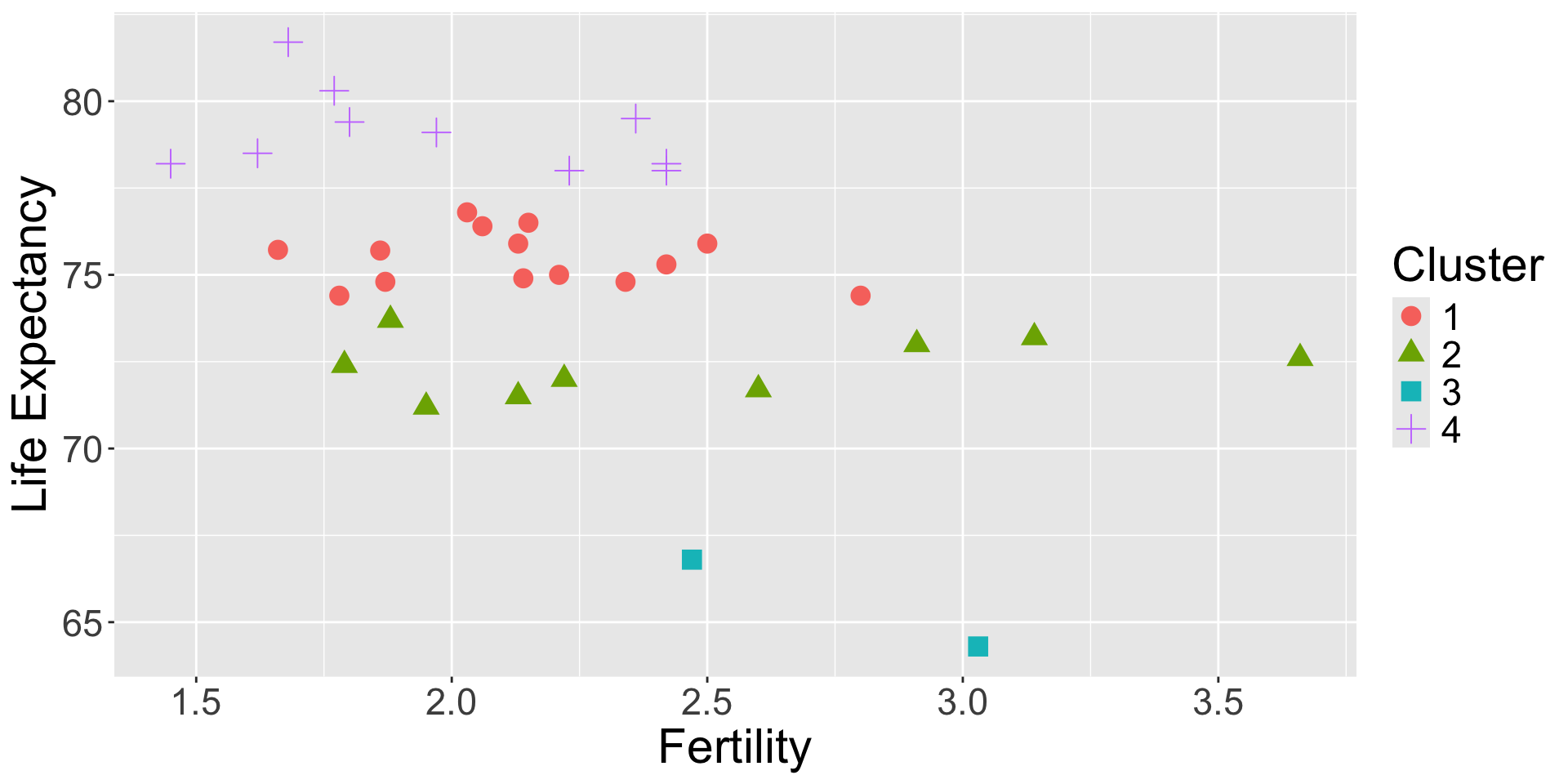
Scatterplot of Fertility vs Life expectancy where shape of each observation is related to their cluster assignment. The overall relationship is moderately negative, with the four clusters grouping observations from top to bottom.

Example: gapminder (3/3)

What if we choose fewer clusters?

k <- 3
kmeans_clusters <- kmeans(gap_fle, centers=k, nstart = 10)
kmeans_clusters$cluster <- as.factor(kmeans_clusters$cluster)

ggplot(gap_fle, aes(x=fertility, y=life_expectancy)) + 
  geom_point(aes(color=kmeans_clusters$cluster, pch=kmeans_clusters$cluster), size = 4) +
  labs(y = "Life Expectancy", x = "Fertility",
       color = "Cluster", shape = "Cluster") +
  presentation_theme
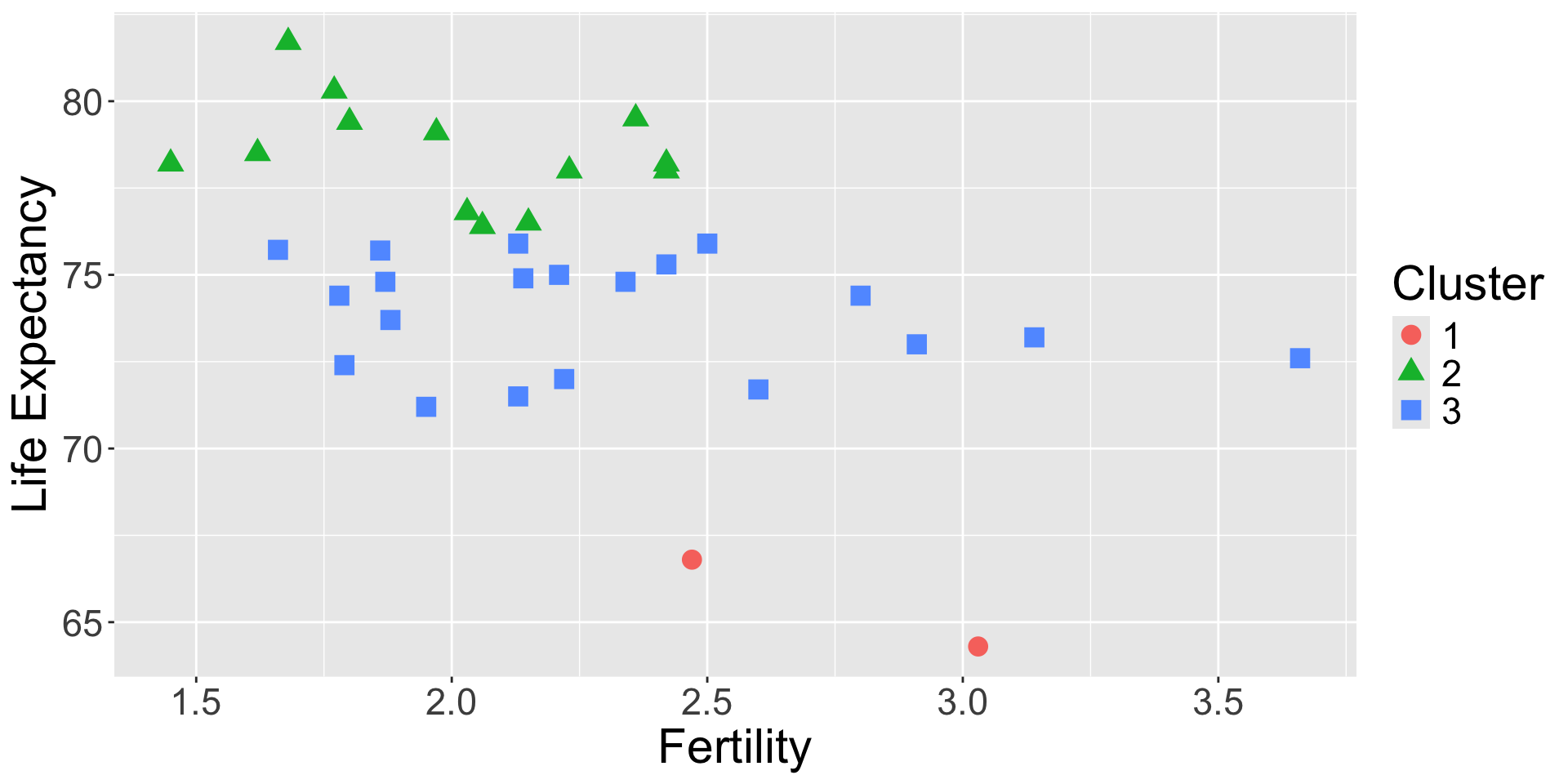
Same scatterplot of Fertility vs Life expectancy as the last slide, but now there are only three clusters. The bottom cluster remains the same, but the top three clusters combine into two.

Agglomerative Clustering

Hierarchical Method: Agglomerative Clustering

  • Doesn’t require pre-specified number of clusters
  • Tree-based representation of observations called a dendrogram
  • Agglomerative (bottom-up) clustering: start from leaves and combine clusters up to trunk.
  • Cut the tree to obtain a specific number of clusters

Hierarchical Clustering: Algorithm

Steps:

1). Define a dissimilarity measure between each pair of observations (usually Euclidean Distance).


2). Iterative:


3). Repeat until all observations are fused together into a single cluster.

Hierarchical Clustering: Algorithm

  • Dissimilarity is difference between two observations

  • Linkage defines dissimilarity between two groups of observations


Output will depend on both linkage method and dissimilarity measure

Example: gapminder

Step 1). Define a dissimilarity measure

  • Two variables: fertility and life_expectancy
  • calculate “distance” for every pair of countries
  • display as distance matrix
gap_fle <- gapminder_2015 %>%
  filter(continent == "Americas") %>%
  select(fertility, life_expectancy, country)

rownames(gap_fle) <- gap_fle$country

gap_dist <- dist(gap_fle[,1:2])

gap_dist_matrix <- gap_dist %>% as.matrix()
gap_dist_matrix[1:4, 1:4]
1
Select just the data we want
2
By default, this uses Euclidean distance
3
This is just to display part of the distance matrix – strictly speaking, this is not necessary for the functions we’re using
                    Antigua and Barbuda Argentina     Aruba  Bahamas
Antigua and Barbuda           0.0000000 0.1345362 0.7889233 2.705993
Argentina                     0.1345362 0.0000000 0.9211406 2.812988
Aruba                         0.7889233 0.9211406 0.0000000 2.031945
Bahamas                       2.7059933 2.8129877 2.0319449 0.000000

Example: gapminder (2/2)

Steps 2 and 3). Cluster observations based on the similarity measure and linkage method - Plot dendrogram

clusters <- hclust(
  gap_dist,
  method = "complete")

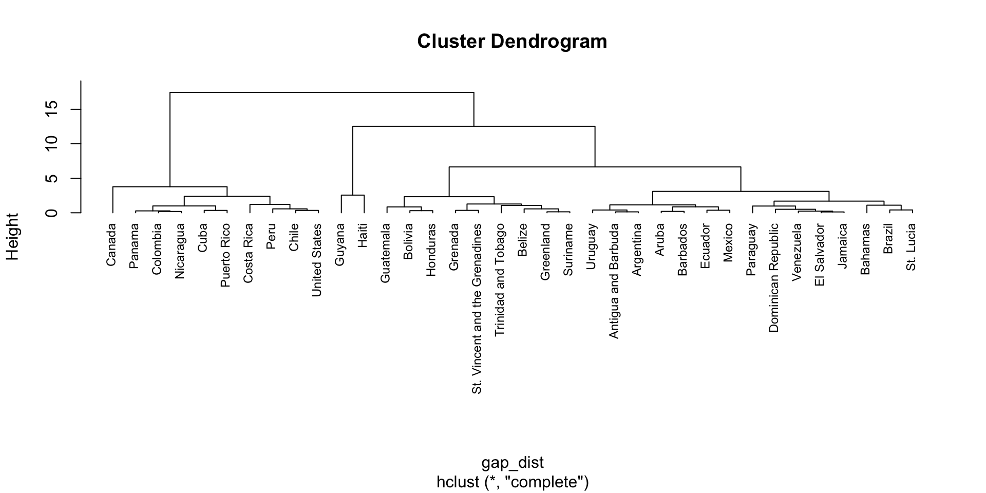
plot(clusters, hang = -1, cex = 0.75)
1
Computed on previous slide
2
linkage method is set to “complete”
Dendrogram for hierarchical cluster of countries using just fertility and life expectancy.

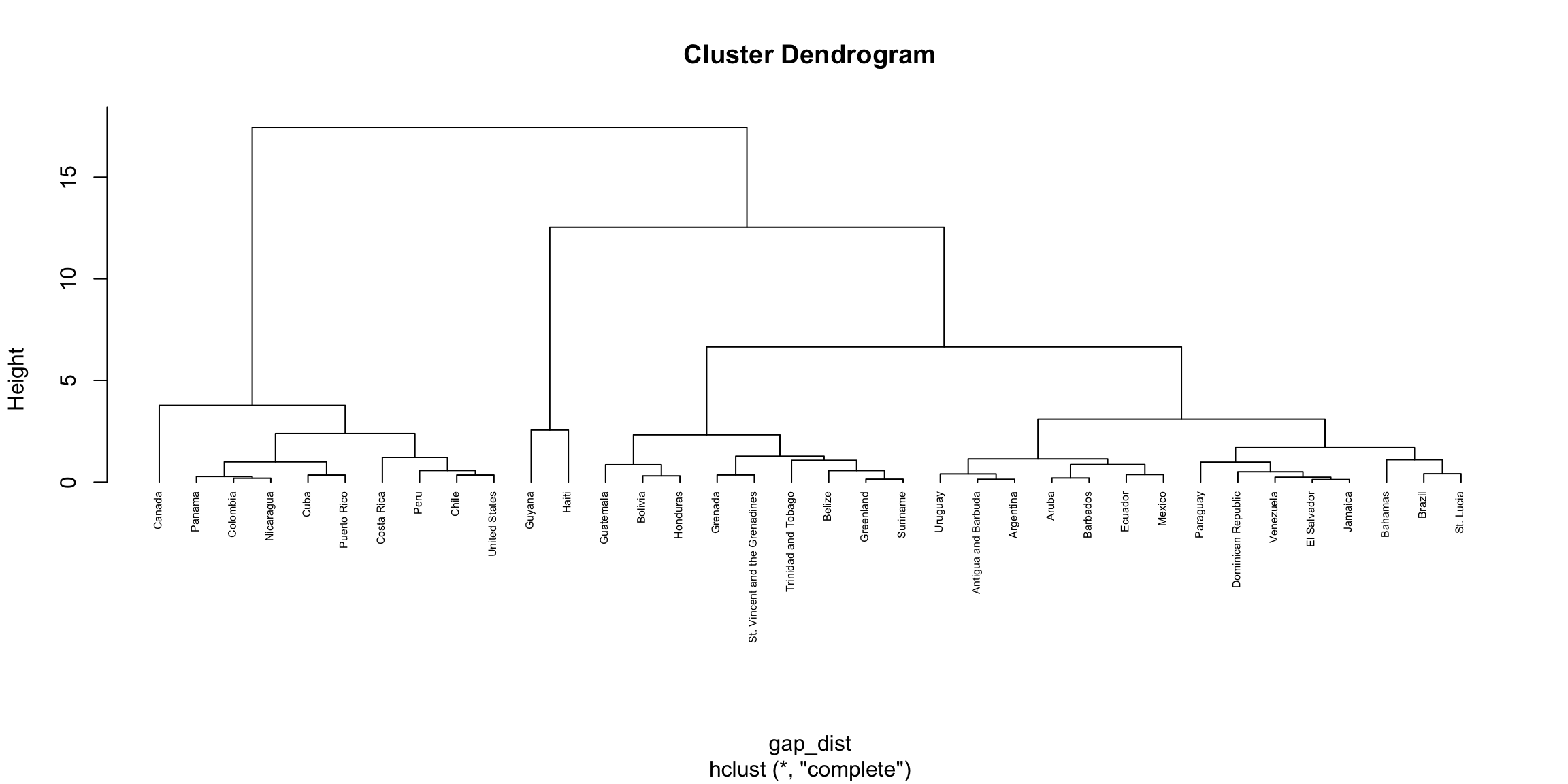
Reading a Dendrogram:

Dendrogram for hierarchical cluster of countries using just fertility and life expectancy. Same dendrogram of previous slide.

Specifying the number of clusters

Obtain a specific number of clusters by “cutting” the dendrogram using the cutree function

clus4 = cutree(clusters, 4)

gap_clusters <- cbind(gap_fle, clus4)
1
Cuts the dendrogram to obtain 4 clusters
2
Combines output from (1) with the data so we can assign each country to a cluster.

Visualize with ggplot gap_clusters %>% ggplot(...) (full code not shown)
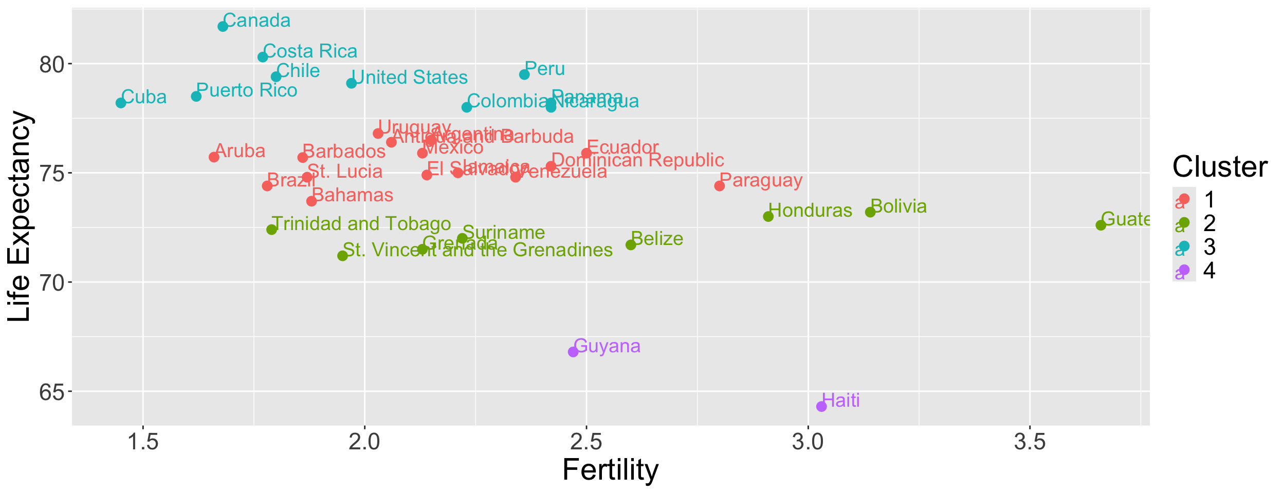
Same scatterplot of Fertility vs Life expectancy as previous, but with only four clusters from hierarchcial clustering. The cluster pattern is similar to k-means with four clusters

Clustering in practice

Practical issues

  1. Try several combinations of options
  • Different values of \(K\) (for \(K\)-means)
  • different dissimilarity/linkage functions
  • where to cut the dendrogram
  • More important than making the right choice1 is documenting why you made the choice you did.
  1. There’s no consensus “best” method fod validating clusters
  • Is the method finding true signal, or just fitting the noise?
  • There are some methods that can give meaningful \(p\)-values, but it’s difficult in general
  1. Clustering methods force every observation into a single cluster.
  • Doesn’t allow for outliers to not belong to any group
  • Doesn’t allow for multiple membership - methods which allow this are called mixture models

Standardizing Inputs

Results can be affected by variables with different scales (see also KNN notes)

Scaling data can mitigate this issue

data_scale = gapminder_2015 %>%
  filter(continent == "Americas") %>%
  filter(infant_mortality != 'NA') %>%
  select(infant_mortality, life_expectancy) %>%
  scale() %>%
  as.data.frame()
1
Same data as previous running examples
2
Scale the data to standardize variables
3
Output can now be used for any clustering method

Summary

Hierarchical clustering:

  • No need to decide the cluster number before the clustering
  • Reproducible result
  • Computationally slow

k-means clustering:

  • Need to decide the cluster number first
  • Randomness may lead to different result
  • Computationally fast

Try It Yourself

Now let’s add a third variable: infant_mortality. Do:

  • K-Means clustering (try with different \(k\) values). Make a data visualization with fertility and life_expectancy.

  • Hierarchical clustering. Decide on the number of clusters that seems appropriate. Make a data visualization with fertility and life_expectancy and compare to your k-means output.

  • Decide if standardizing your inputs is necessary. If so redo the two steps above and compare your results.